
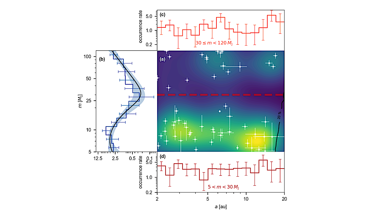
Distribution of companions in semi-major axis and mass, along with the occurrence rate density of subsamples. (a), Detection efficiency-weighted KDE and distribution of our sample (white points). We divide the

Distribution of companions in semi-major axis and mass, along with the occurrence rate density of subsamples. (a), Detection efficiency-weighted KDE and distribution of our sample (white points). We divide the

A view of the outside of the OSIRIS-REx sample collector. Sample material from asteroid Bennu can be seen on the middle right. Scientists have found evidence of both carbon and

The Alvin submersible is recovered on deck following a seven-hour dive, concluding a successful day of hydrothermal vent sampling. Photo courtesy of Will Carter Imagine descending nearly a mile and
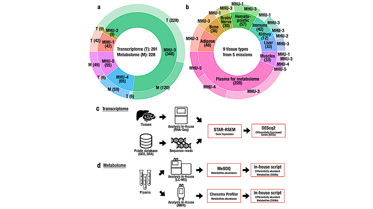
Overview of the ibSLS database content. a. Numbers of samples available in the current ibSLS, categorized by assay type (outer ring) and mission (inner ring), with sample counts indicated in
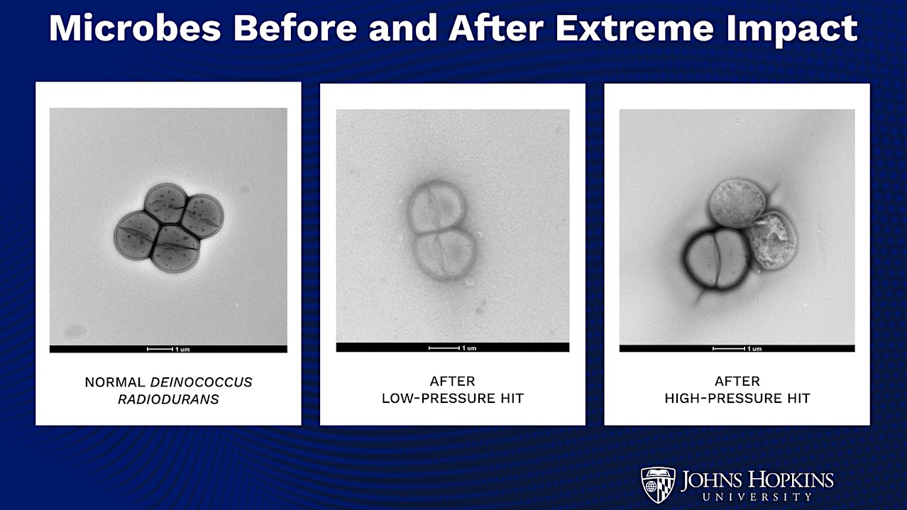
Tiny life forms tucked into debris from an asteroid hit could catapult to other planets – including Earth – and survive, a new Johns Hopkins University study finds. The work
Distribution of companions in semi-major axis and mass, along with the occurrence rate density of subsamples. (a), Detection efficiency-weighted KDE and distribution of our sample (white points). We divide the
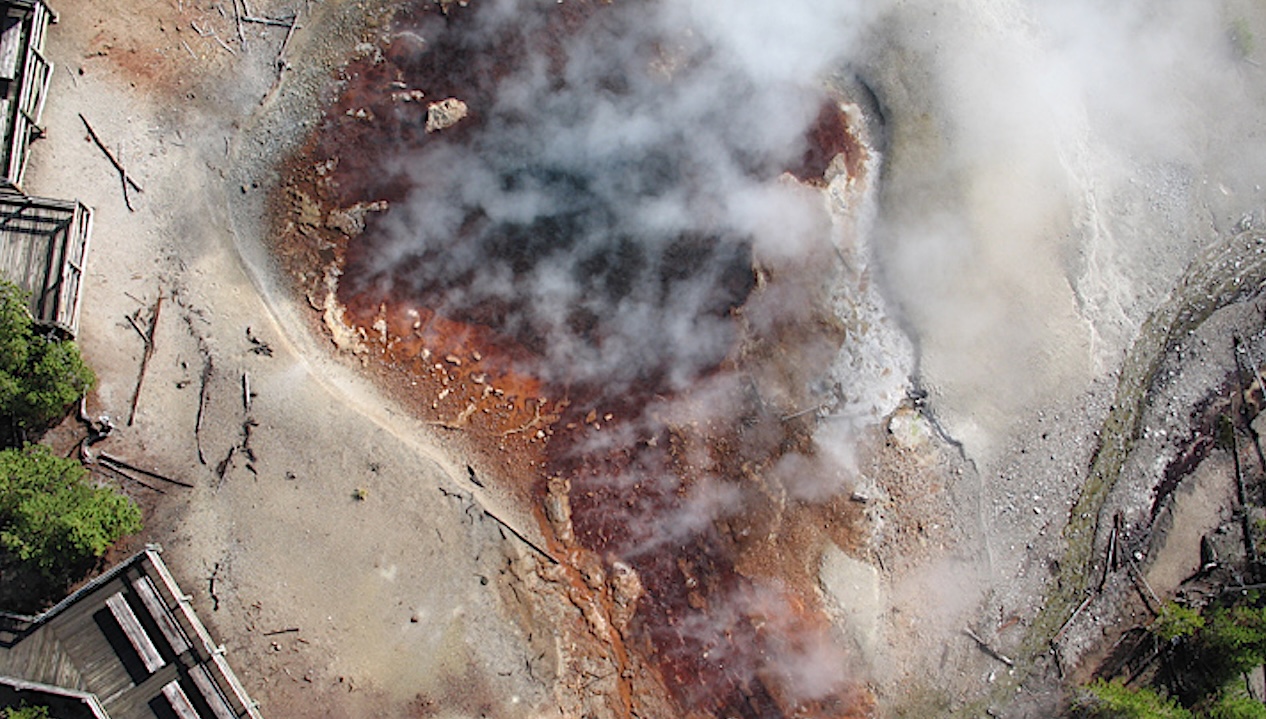
This geyser exhibits irregular behavior, sometimes erupting regularly for months, and then ceasing altogether. Echinus is a rare acidic geyser, with a mixed water rich in both sulfate and chloride.
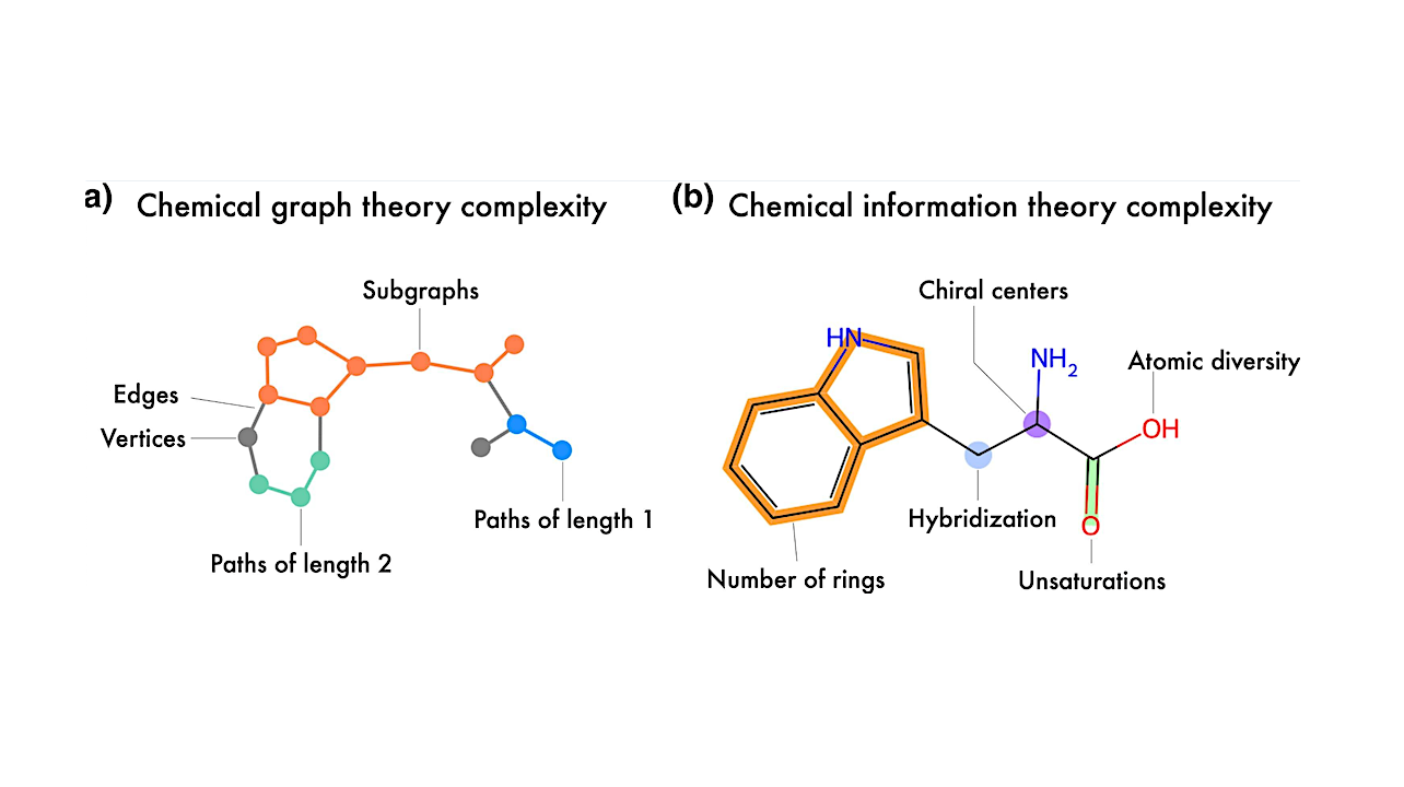
Representation of the two main frameworks used to quantify molecular complexity: (a) graph-theoretic and b) information-theoretic approaches. Tryptophan is depicted as both a graph representation and a molecular structure, illustrating
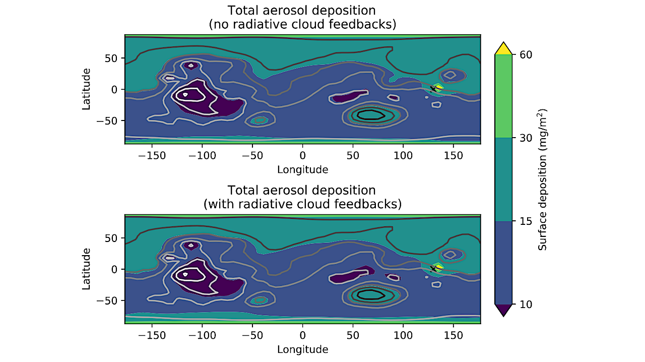
Aerosol deposition on the surface following 5 Mars years of 2.5 l/s release and 15 Mars years of shutoff. The distribution is comparatively uniform, with more deposition at low elevations,

Occurrence of bd-type oxygen reductase in a dated tree of life. Branches in the dated tree of life obtained from Mahendrarajah et al. are colored according to the